Building a DCF model in Google Sheets

Discounted Cashflow models are immensely popular methods in company valuation, where estimates of future cash flows are discounted back to the present day. This method is based on the principle that the oracle Warren Buffett has mentioned many times: "The value of a business is the sum of all the cash it will generate in the future". Of course, the future is uncertain, and the DCF model is only as good as the assumptions you make, and can be subjective based on the inputs you use.

Being said, in this blog piece we'll take a look at building both an automated, using SheetsFinance functions, and a manual option for you to add custom inputs. Note that the automated option is a great way to get started, but as you get more confident in your own financial research, you may want to add more custom inputs to make the model more accurate or fine tune it to your needs.

Getting Started with SheetsFinance

1. Make sure SheetsFinance is properly installed and linked to your google account, if not, you can find how to do so here.
2. Get access to the template here
3. Want to learn through a video tutorial? Check out our Youtube Channel.

Building up the Inputs Sheet

Before we even begin calculating the DCF, we need to gather some information about the company we are valuing. This includes the company's financials, growth rates, and discount rates. Let's create a sheet specific for these inputs, and add a helpful dropdown to toggle between the manual and automated options.

Let's place the ticker symbol in cell A3, and the latest year in cell A5, we'll use these cells to fetch directly with our SF() functions. Note we've ignored the entire row A to keep it clean (filled in black and reduced to a small size to act as a boundary), but you can use it for other purposes! Let's add some colour coding for cells so we know which cells are for editing and which are not.

Next up is adding in a dropdown in cell E2, with options "Yes" and "No". This dropdown will be used to toggle between the manual and automated options. Note that we've also added a simple text box to indicate what this "button" does.

Perfect! Let's move on to the next step, and that is our actual inputs, which are the following:

• TTM EBITDA
• TTM Free cash flow
• EBITDA Growth Rate
• FCF Growth Rate
• Discount Rate (WACC)
• Terminal Value Multiple
• Margin of Safety
• Time Period

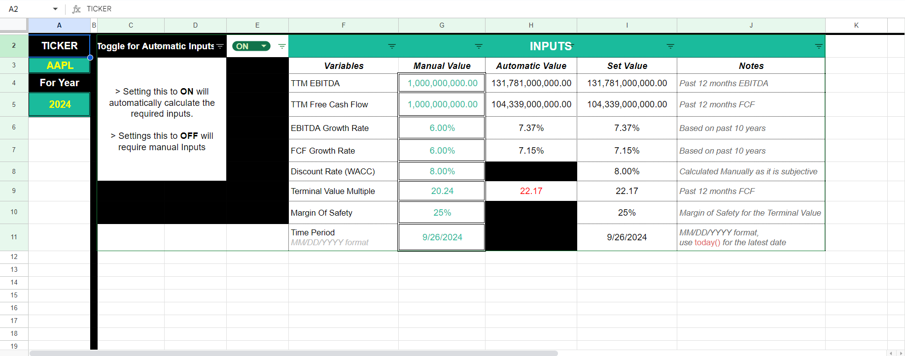
Let's add these in cells F4:F11, and draw out two columns aside to add the manual and automated options. We'll use the SF() functions to fetch the data for the automated option, and the user can input the data for the manual option.

Going back to our latest year cell A5, let's change its value to:

    =Year(Inputs!$I$11)
    

Before we jump into the automated column, lets add the Set Values column, which will output either the manual or automated cell along its row, depending on the dropdown selection. We'll use the IF() function to do this, and the formula will look like this:

    =IF($E$2="ON",H4,G4)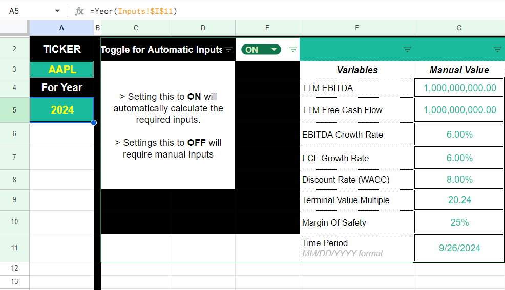
    

Note: We've also added a final column to note down some key assumptions, which you can view yourself in the attached image below, or by heading to the template itself!

Fetching the Data

To generate the TTM EBITDA value, we'll use the following function:

    =SF($A$3, "historicalFinancialsIncomeTTM", "ebitda",Inputs!$I$11,"NH&NLI&sum")
    

💡 Quick Tip: Adding sum as part of the final options parameter will sum the past 4 quarters relative to the specified date generating the TTM EBITDA with reference to that date. Also note that we are excluding any headers or line items using NH&NLI. Find out more about the TTM Reports for financial statements here

We'll apply similar logic to fetch the TTM Free Cash Flow, with:

    =SF($A$3, "historicalFinancialsCashTTM", "freeCashFlow",Inputs!$I$11,"NH&NLI&sum")
    

Before we jump into calculating the growth rates, it's important to highlight that WACC, Margin of Safety, and Time Period, are all subjective and up to you as an investor to decide. There are of course different, common methods to calculate certain items such as the WACC but this will depend on your own preferences. Therefore, the cells in the automated data column for these variables are left empty and the default option in the Set Values column is set to the manual. We recommend you apply a Margin of Safety of at least 10%. As Benjamin Graham has said, risks are involved when purchasing a security, and finding stocks at a price significantly lower than its intrinsic value is important to both enhance potential returns, but mainly to reduce the risk of loss on the investment through incorrect assumptions and human mistakes.

💡 Quick Tip: Spend some time getting an understanding of how the cost of equity and cost of debt impact the WACC (Weighted Average Cost of Capital) calculation. WACC essentially highlights the cost of financing for a company given its position in Total Equity against Long Term Debt, and the costs implied with both of these. The WACC is a crucial input in the DCF model, as it is used to discount the future cash flows back to the present day and taking the time to get an accurate figure is very important.

Let's look at the Growth rates, which we'll do through an additional sheet called Data Page. Here we fetch the past decade's worth of EBITDA and Free Cashflows, and calculate this retrospective change, assuming it will apply to the future. Note again that this is an unrealistic assumption, the future is never the exact same as the past and this is why we apply an adequate Margin of Safety to compensate for our lack of ability to predict the future.

Use the following to generate the past 10 years in EBITDA:

    =SF(Inputs!$A$3,"historicalFinancialsIncome","ebitda",$K$3&"-"&$B$3,"NH&-NLI")
    

And for the Free Cash Flows:

    =SF(Inputs!$A$3,"historicalFinancialsCash","freeCashFlow",$K$3&"-"&$B$3,"NH&-NLI")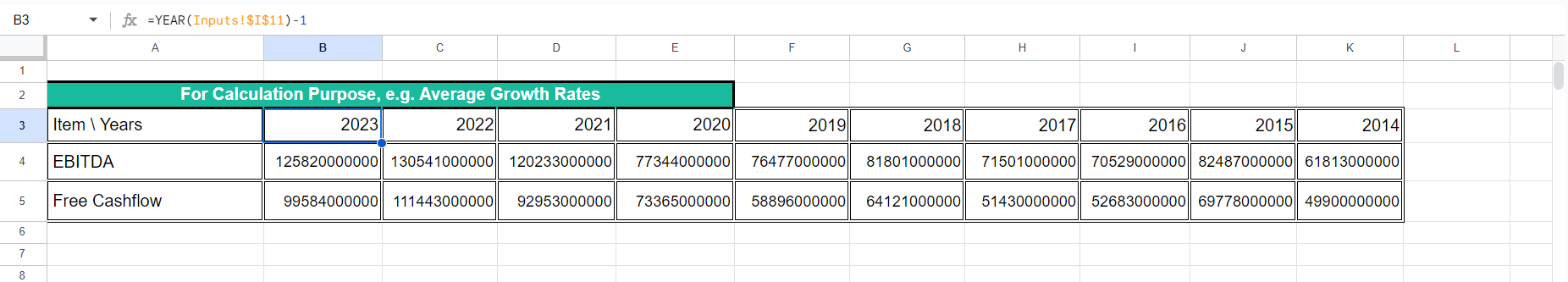
    

From the image above, note that we've actually define the latest year using:

    =YEAR(Inputs!$I$11)-1
    

Finally, heading back into the Inputs Sheet, we'll calculate the growth rates for EBITDA and Free Cash Flows. We'll use the following formula for EBITDA to compute the 10 year exponential growth rate:

    =(('Data Page'!B4/INDEX('Data Page'!B4:K4, 10))^(1/10)) - 1
    

And similarly, for the Free Cash Flow, just drag the above cell equation down to the Free Cash Flow row:

    =(('Data Page'!B5/INDEX('Data Page'!B5:K5, 10))^(1/10)) - 1
    

The final variable that we know need to look into is the Terminal Value Multiple, which in our case is simply the Enterprise Value divided by the latest EBITDA. Why this metric? There are a number of ways to define the Terminal value but our argument is that the enterprise value of a company is a more stable form of computing a company's net worth, and we're already using EBITDA for all our other calculations. We can fetch this Terminal Value from the Ratios function native to SheetsFinance with:

    =IFERROR(SF($A$3, "ratios", "enterpriseValueOverEBITDA",YEAR(Inputs!$I$11)),SF($A$3, "ratios", "enterpriseValueOverEBITDA",YEAR(Inputs!$I$11)-1))
    

🔥 Hot Tip: From the above, we added an IFERROR() statement in case the latest year's data is not available, and instead fetch the previous year's data. This is a good practice to ensure that the model doesn't break if the latest year's data is not available.

And that's our Inputs Sheet done! We've fetched all the necessary data, and now we can move on to the DCF Valuation Sheet.

Building the DCF Valuation Sheet

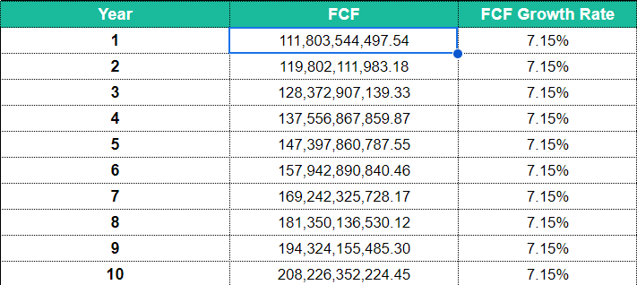
Let's first model out the next 10 years of EBITDA and Free Cash Flows, which we'll do by using the growth rates we calculated in the Inputs Sheet. Let's draw out a column with the year number, then one for Free Cash Flows, and the associated growth rates which we can fetch using:

    =Inputs!$I$7
    

Note: You can manually change the growth rates along this column to see how it affects future Free Cash Flows, or if you have a specific growth rate in mind for future years.

Then simply compound the most recent Free Cash Flow figure within an incremental time period, from 1 to 10, and you'll have your future Free Cash Flows.

For example, for the first Free Cash Flow cell, we can use the following formula:

    =(Inputs!$I$5)*(1+$E13)^($C13)
    

Note that the above references the TTM Free Cash Flow from the Inputs Sheet, and the growth rate from the DCF sheet, we then compound that rate up to the year number. Repeat the same procedure for the cells below until you forecast the next 10 years.

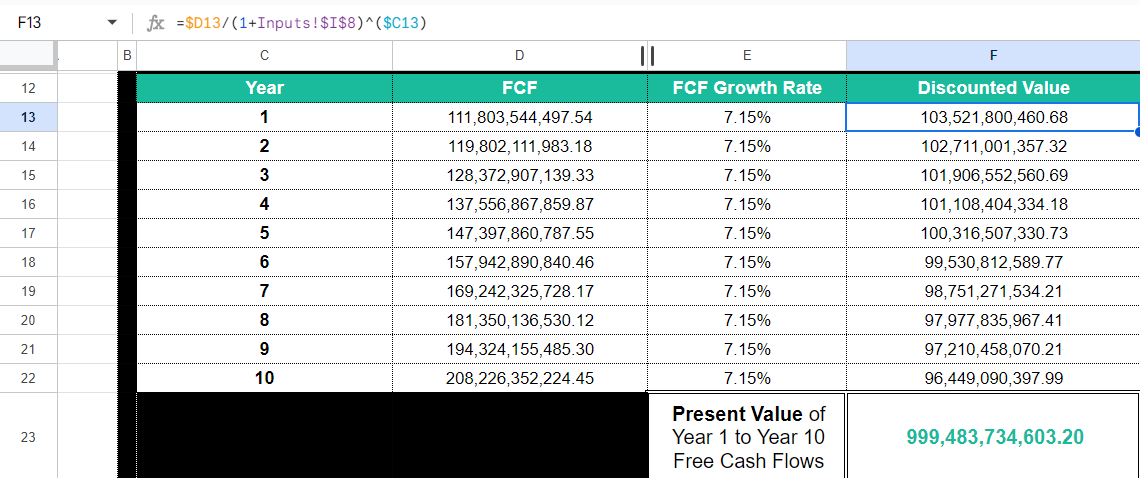
Given that we've now forecasted the next 10 years worth of Free Cash Flows, we need to consider the time value of money, i.e. let's discount these free cash flows back to today, using our WACC figure.

    =$D13/(1+Inputs!$I$8)^($C13)
    

As before, the code above takes in the calculated Free Cash Flow for the year and discounts it back to the present day using the WACC figure (reverse compounding). Repeat this for the full 10 years and then sum them all up to get your discounted Free Cash Flows.

To forecast the EBITDA over the next 10 years, repeat the exact same steps except now use the EBITDA growth rate and the most recent TTM EBITDA figure. Then discount them in the same manner as we did for the Free Cash Flows, using the following to forecast the EBITDA year by year:

    =(Inputs!$I$4)*(1+$H13)^($C13)
    

Make sure to add two additional columns on the right to fetch the growth rate, i.e. using:

    =Inputs!$I$6
    

And then discount back to the present day:

    =$G13/(1+Inputs!$I$8)^($C13)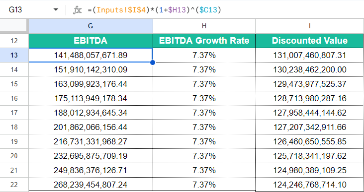
    

We now need to calculate the Terminal Value, which is the value of the company at the end of the forecast period.

To do so, we'll fetch the Terminal Value from our Inputs Sheet and multiply it by the discounted EBITDA value forecasted for Year 10 (the end of our forecast). This is where our Margin of Safety now comes in which we apply to the final discounted EBITDA value in Year 10. This is to ensure that we are not overpaying for the company, and that we are taking into account the risks involved in investing in the company.

We use the following to compute the Terminal Value, where F24 comes directly from the Inputs sheet as the initial Terminal Value, and I22 refers to our Year 10 value for the discounted EBITDA.

    =F24*I22*(1-Inputs!$I$10)
    

The final part of the equation is to take away, or subtract, the Net Debt of the company. Why? If you were to acquire the entire company, you would also be acquiring its debt, which would come at an expense to you and so should be excluded from the actual underlying valuation of the company (i.e. you'd want to pay less for something that comes with a debt burden).

We'll apply the following =SF() function to fetch the Net Debt for the latest year, with a failsafe mechanism if the data is not available by reading the next most recent year's data:

    =IFERROR(SF($A$3, "historicalFinancialsBalance", "netDebt", Year(Inputs!$I$11)),SF($A$3, "historicalFinancialsBalance", "netDebt", Year(Inputs!$I$11)-1))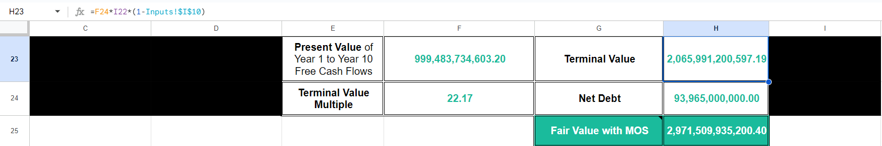
    

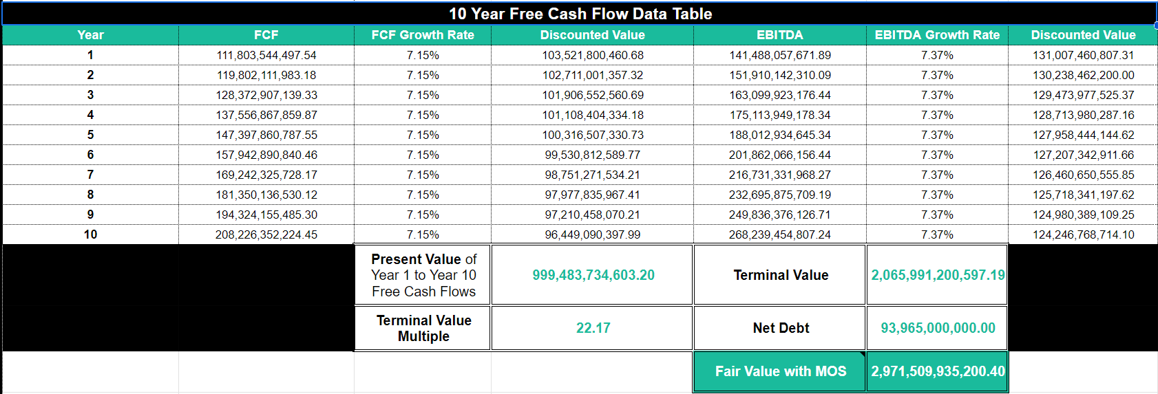
That completes the DCF Valuation table for the company! 🎉

You can now see the present value of the company, and compare it to the current market capitalization to see if the company is undervalued or overvalued.

Let's have a final look at the DCF Valuation table.

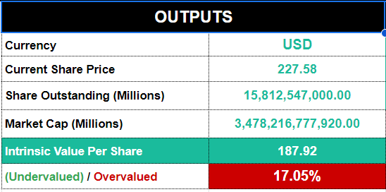
You can now fetch the current market capitalization of the company, and compare it to the DCF valuation to see if the company is undervalued or overvalued. Or, if you prefer comparing on a share price basis, import the current outstanding number of shares and divide the DCF valuation by the number of shares to get the intrinsic value per share. This value could then be compared to the current share price, like so:

⚙️ Get The Template: Feel free to check out the template right here, it's free to use and modify to your liking 🙂.

Using the Function Generator to Build these Functions for You

Feeling a bit overwhelmed by all the functions? Don't worry, we've got you covered 😁

Our Function Generator is a tool that builds these functions for you. Just select the function you want to use, input the required parameters, and the Function Generator will generate the function for you and automatically insert it into your Google Sheet. You can find the Function Generator in the Google Sheets under (Extensions > Sheets Finance > Function Generator).

Finding the Correct Ticker Symbol

Want to run this DCF on your favourite companies. Find the correct ticker symbol by using our Symbol Search tool within Google Sheets (Extensions > Sheets Finance > Symbol Search), or online on our Symbol Search Page.

You can also use the SF_MAP function to translate any ISIN, CUSIP or CIK code into the correct ticker used at SheetsFinance.